Managing SharePoint List Permissions

I typically don’t do a lot in Microsoft SharePoint, however on my current project I’ve been working on building out a little site that has required learning some new things about it. In particular, I had a main site, with multiple lists on the site. I also have multiple groups of people setup and I wanted to ensure that each group can view the main site, but then can only view their specific list.

So it turns out that if you create a group at the site level than it automatically overrides permissions at the list level, even if you tell a list to not inherit permissions from the parent site. What you have to do is create a group at the site level but do not select any of the permission levels, just create the group without any permissions. This will create the group with “Limited Access” permissions that does not allow them to view or do anything.

Then, you go to the specific list you want to grant the group permissions to and add the group there, granting them permissions directly at the list level. In my case, I gave them “View Only” permissions because it allows users to view lists and look at documents attached to the list.

Finally, in order for users to view the main site (but not any lists below the main site), create and add them to a Visitor’s group that you grant “Read” permissions too. This restricts them to view the site, but not view any lists (besides the specific ones you grant permissions too).

Hope this helps!

The two Microsoft help articles I referenced are:

Remove users and groups from site access – Windows SharePoint Services

Customizing user access to a SharePoint list or library – SharePoint Server

Excel: How to use the INDIRECT function – Example

I received a request for a follow-up post to my last post on how to use the INDIRECT function in Excel. The request was to create a sample table showing a potential setup and use of it.

The best use I’ve found for the INDIRECT function is to build dashboards. You can have all your data stored on one sheet and then use INDIRECT formulas in combination with others to pull over only the data you want in a quick and easy manner.

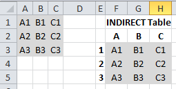
In the picture below, there are two sample tables. The one on the top left is my “Original Data Table” which could be stored on any tab. The “INDIRECT Table” on the right uses INDIRECT formulas to pull over the data from the first, original table.

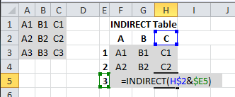
Remember that the INDIRECT formula takes in a text string and converts it to a cell reference. In this case, I put my column references as table headers and my row references as row IDs for my INDIRECT table. In this second picture, you can see how I combine the column reference & row reference in my INDIRECT formula to create a formula that is easily copied over to all the other cells in my table.

With properly setup column & row references, I need only write a single INDIRECT formula to pull over all my data in the correct order. I could just have easily made it skip every other row or skip a couple of columns, or even reorder the columns or rows by reordering my column & row references. My INDIRECT formula wouldn’t have to change at all!

Hope this helps! Let me know if you have any further questions.

Thanks!
~Yosef

Excel: How to use the INDIRECT function

The Excel INDIRECT function is useful for displaying data in another cell by passing it text strings to tell it where the value is.

The syntax for the Indirect function is as follows:

INDIRECT(ref_text,[a1])

Where:

ref_text is a text reference to another cell & [a1] is a logical value that specifies what type of reference style ref_text is using.

In excel you have two types of cell reference styles:

1. A1 style is where each row has a number and each column has a letter (the default view in excel).
2. R1C1 style is where each row has a number and each column has a number.

A1 is indicated by [a1] = “TRUE”, R1C1 is indicated by [a1] = “FALSE” in the INDIRECT formula.

For example in order to display a specific column of data in a given row (in this example, row 7), the following function is used:

=INDIRECT($B$1&$A7,TRUE)

The first argument, $B$1&$A7 concatenates the values in cell B1 & A7 together to create a text statement of where the data that needs to be displayed is stored. In this case B1 = “Data!B”, A7 = 3 so the final result is “Data!B3” so the value displayed in the cell is the value on the Data tab in the B3 cell.

Column A now displays the row of the data for that particular project on the “Data” tab.

Hope you find this useful!

~Yosef