Setting Default PivotTable settings in Excel


Microsoft’s latest update to Excel now allows you to set defaults for how you want your PivotTables formatted. As someone who builds PivotTables all the time & 98% of the time want them setup the same way – this is a huge help!

To access the default options, open Excel and go to: File > Options > Data > & click on the Edit Default Layout button.

If you have an existing PivotTable that’s setup the way you want, simply use the Layout Import option at the top of the window to select the existing PivotTable and import the options all ready set.

The options I have set are:

  • Subtotals: Do Not Show Subtotals
  • Grand Totals: On for Rows and Columns
  • Report Layout: Show in Tabular Form
  • repeat All Item Labels: Checked box

In addition, click the PivotTable Options button and you can optimize all your PivotTables moving forward (huge file size saver!).

Select the Data tab and select/unselect the following options:

  • Save source data with file: Unchecked
  • Enable show details: Checked
  • Refresh data when opening the file: Checked
  • Number of items to retain per field: Select the None option

This will force excel to refresh the PivotTable every time the file is opened but it will also not save the source data (calculations behind the PivotTable) which makes the file size much smaller & less susceptible to file corruption.

Enjoy!
~Yosef

Building Dynamically Driven Excel Hyperlinks


I recently came upon a challenge that at face value looked straight forward but actually proved to be quite tricky.

What I wanted to do was create a drop-down menu in Excel. Depending on the choice selected, a hyperlink would be created that would allow you to “jump” to a specific location in the Excel workbook based upon your selection.

The solution I hit upon is to use the Hyperlink formula with a unique twist.

First, I created two different worksheets – for this example I’ve creatively named them “Test Sheet 1” & “Test Sheet 2”.

Next, I created a drop-down list menu using the two worksheet names (cell C2 in picture below; see my previous post for details: Excel: Creating a Drop Down Menu).

Excel: Drop Down Menu Example

Finally, in cell C4 I put the following formula =HYPERLINK("#'"&C2&"'!A1","Go to "&C2) where the first part "#'"&C2"'!A1" builds the actual link #’Test Sheet 1′!A1 or #’Test Sheet 2′!A1 (depending on the drop down selection) that takes you to the A1 cell on either the Test Sheet 1 or Test Sheet 2 worksheet, and the second half "Go to "&C2 builds the text that’s displayed to the user in cell C4.

Excel: Dynamic Hyperlink Formula

Viola! Depending on the drop down item selected, the hyperlink will dynamically update and direct the user to the correct worksheet.

The tricky part was in figuring out where to put all the single & double quote marks as well as learning about using the hash mark to indicate that the URL was inside the current workbook without having to specify the full name of the workbook.

This should come in handy when building table of contents, forms, &/or surveys in Excel.

~Yosef

Excel PivotTable Slicer Options Explained


Microsoft has a great tutorial on how to use slicers to filter PivotTable data and I don’t feel that I need to duplicate their tutorial here. You can read all about it here: Microsoft: Use slicers to filter PivotTable data

What the article does not cover is the Slicer settings available by right-clicking on a slicer and selecting that bottom option “Slicer Settings”.

There are 3 main settings that you can set here – I typically only change the last one and leave the rest on their default settings. They are:

  1. Name – this is the name by which you can refer to the slicer in formulas. I typically just let this be the default. (e.g. CUBERANKEDMEMBER("PowerPivot Data",Slicer_Name,ROW()))
  2. Header – this is the name displayed above the slicer. You can choose to turn it on or off and customize the name if needed. Again, I typically just leave the header visible with the default name.
  3. Item Sorting and Filtering – Here’s where you can choose to:
    • order the values ascending or descending
    • Perhaps most important for visual aesthetics (and the value I typically choose to modify most often) you may hide items with no data
    • Choose to visually indicate items with no data (by making them more transparent)
    • Choose to show items, which have no data associated with them, last in the list
    • Continue to show items which have been deleted from the original data source table

Questions? Suggestions? Leave a comment!

Intro to the Excel VBA Editor


This post is not about learning to code, it’s about where to find your way around the basics of the Excel VBA developer interface. If you’re just getting started with VBA programming, this should help give you an idea of where to find the tools you need.

The topics we are going to cover today are:

  • How to enable the Developer tab in Excel 2007 and up
  • How to access VBA code and where to store your code
  • How to access the VBA macro recorder and why it’s useful
  • How to insert buttons in your spreadsheet and assign code to them
  • How to use the Immediate window
  • The (common) Run, Debug, & Tools menu options

After reading this, you’ll be ready to begin focusing on learning to code!

How to enable the Developer tab in Excel 2007 and up

  1. The first thing you need to do to access the VBA editor in Excel is to enable / display the Developer tab. To do this, click the Office circle or the File tab and click on the Options button.
  2. Click on the Customize Ribbon option on the left hand side of the window.
  3. Ensure that the check-box is selected for the Developer option on the right hand side.
  4. Excel_Ribbon_Options

  5. Click the OK button.
  6. You should now see the Developer tab appear on the right hand side of the Ribbon bar.

How to access VBA code and where to store your code

  1. Once you have access to the Developer tab, select it and then click the Visual Basic button on the right hand side in the Code section.
  2. Excel_Developer_Ribbon

  3. This will open up the VBA editor window.
  4. On the left hand side, you will see a basic Project tree structure that shows the different worksheets in your workbook, as well as any code modules, or other Excel objects. On the right hand side, you will see the basic (probably empty) code window where you can write VBA code.
  5. Typically, I like to create one or more modules for storing my code. I will usually have one module for my main code routine, one for any functions I may call, and one or more for large subroutines. How you structure your code is up to you. You can also store your code in the specific worksheet that you want to call it from.

Excel_VBA_Window

Excel_VBA_Insert_Module

How to access the VBA macro recorder and why it’s useful

  1. On the Developer tab, there is a VBA macro recorder.
  2. Excel_VBA_Record_Macro

  3. Clicking on it, Excel will prompt you for what to call the macro and then will begin to record (in VBA code) all the clicks and keystrokes that you make as you manually update your worksheet.
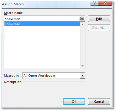
  4. Excel_VBA_Assign_Macro

  5. This can be extremely helpful to help you quickly prototype basic code, or to figure out what the options are for using VBA to manipulate your worksheet. For example, you could manually apply a filter to a Pivot table, then see what the macro recorded to figure out what the code is for doing this programmatically.
  6. The macro does have limitations – for example, it won’t construct any code to iterate through a job. It will construct code to do the action over and over (i.e. copy the code multiple times, potentially making for a HUGE amount of code, but you will need to learn how to build a If, For, or When loop to iterate through the action multiple times.
  7. When you click the Stop Recording button, it will save the code to a new code module in the VBA code editor.

How to insert buttons in your spreadsheet and assign code to them

  1. You can add a button to your spreadsheet that when clicked, will run specified VBA code.
  2. To do so, click the Insert button in the Controls section. Click on the square box icon in the Form Controls section. Then click and “draw” a button where ever you want it on your spreadsheet.
  3. Excel_VBA_Form_Controls

  4. As soon as you finish drawing the button, Excel should prompt you to assign a macro to the button. All subroutines that you have created in the VBA editor should appear in a list, available for your selection.
  5. Excel_VBA_Button

  6. You can right-click on the button and choose to edit it, this will allow you to edit the text on the button as well as move it.

How to use the Immediate window

  1. Going back to the VBA editor window, sometimes when you run code, you just want to see the output right away and not have it affect anything in your Excel spreadsheet. This is especially useful for debugging code.
  2. In the example below, a subroutine called showcase defines a variable num as an integer value and then assigns the value of 2 + 2 to the variable num. Then, using the Debug.Print function, the value of num is displayed in what is called the Immediate window (i.e. the value of num is 4).
  3. Excel_VBA_Immediate_Window

  4. If the Immediate window is not visible, you can quickly display it using the shortcut key

The (common) Run, Debug, & Tools menu options

The following is a synopsis of the Run, Debug, & Tools menu options:

The Run Menu

Excel_VBA_Run_Menu

  1. The run menu gives you access to the play, pause, stop functionality of running your VBA code.
  2. The most useful thing to note here is if you click on a subroutine or function with your mouse, you can then use the F5 key to run that specific subroutine.
  3. Also note, if you run code and it breaks, prompting you to enter debug mode, the way to exit debugging is to use the Reset button

The Debug Menu

Excel_VBA_Debug_Menu

  1. When you finish writing your code, click the Compile VBAProject button. Compiling converts the code written in the editor into code that can be read by the Windows run-time environment. If you don’t compile your code, than it is automatically done when the code is run. If the code won’t compile then it needs to be debugged and won’t run until it is fixed.
  2. The other useful thing to note here is the Step Into (F8) option. This allows you to step, one line at a time, through your code.

The Tools Menu

Excel_VBA_Tools_Menu

  1. On occasion, some of your code may require access to other VBA functions that are not typically in Excel. For example, you run VBA code in Excel that also programmatically manipulates something in Outlook or Word. You will need to add a reference to the Outlook or Word functions by using the References option available here.

Hope this helps!
Questions? Comments? As always, let me know in the comments below.

Project Date Calculations in Excel


A relatively common demand management question I’ve been asked to solve in Excel numerous times is how do I figure out how much time is a person allocated to a project during a certain month?

The answer is relatively simple but requires a visual aid to help figure out the logic of the different scenarios:

Project Date Scenarios

As you can see – there are 4 cases that can occur. Our goal is to write an IF statement that models all of these scenarios.

Ta Da! Here you go:

=IF(AND([Project Start]<[Month Start],[Project End]>[Month End]),1,
IF(AND([Project Start]<[Month Start],[Project End]<=[Month End],[Project End]>=[Month Start]),(NETWORKDAYS([Month Start],[Project End])/NETWORKDAYS([Month Start],[Month End])),
IF(AND([Project Start]>=[Month Start],[Project Start]<[Month End],[Project End]>[Month End]),(NETWORKDAYS([Project Start],[Month End])/NETWORKDAYS([Month Start],[Month End])),
IF(AND([Project Start]>=[Month Start],[Project Start]<[Month End],[Project End]<=[Month End]),(NETWORKDAYS([Project Start],[Project End])/NETWORKDAYS([Month Start],[Month End])),0))))

Let's break this down line by line.

=IF(AND([Project Start]<[Month Start],[Project End]>[Month End]),1,

translated is case #1 and it would give us a full 100% allocation during that month.

IF(AND([Project Start]<[Month Start],[Project End]<=[Month End],[Project End]>=[Month Start]),(NETWORKDAYS([Month Start],[Project End])/NETWORKDAYS([Month Start],[Month End])),

translated is case #2 (Project End is either before or equal to Month End), we then find the number of work days between month start & project end and then divide by the number of work days in the month to find the percentage of allocated time.

IF(AND([Project Start]>=[Month Start],[Project Start]<[Month End],[Project End]>[Month End]),(NETWORKDAYS([Project Start],[Month End])/NETWORKDAYS([Month Start],[Month End])),

translated is case #4 (Project Start is after Month Start and before Month End, find the number of work days between Project Start and Month End divided by the total number of work days in the month.)

IF(AND([Project Start]>=[Month Start],[Project Start]<[Month End],[Project End]<=[Month End]),(NETWORKDAYS([Project Start],[Project End])/NETWORKDAYS([Month Start],[Month End])),0))))

translated is case #3 (Project Start is after Month Start and before Month End and Project End is before Month End, find the number of work days between Project Start and Project End divided by the total number of work days in the month.)

Using this formula, you can find (per month, or any other given date range such as an entire year) what percentage of time the project takes up within that date range. This percentage can then be used to calculate number of hours, cost of project, etc.

If you have a specific use case you are interested in getting help with let me know!

~Yosef

Help! Why won’t my Excel formula calculate?!


Note: These instructions are based off Excel 2010 but are applicable for Excel 2007 through Excel 2013 (Office 365).

Has someone sent you a spreadsheet or perhaps you’re working on one and all of a sudden your formulas look like formulas and won’t calculate? Here are the top solutions I have come across for fixing this common error.

  1. Cell text formatting is set to “Text” – If the formatting of the cell has been set to Text instead of General or some other format, the cell will not calculate because it assumes that anything in the cell is text and not a formula. Change the formatting of the cell by pulling down on the drop down in the Number section on the Home tab of the menu ribbon
  2. Excel Number Format

    Excel Number Format Expanded

  3. Show Formulas (Ctrl + ~) has been selected / pressed – If the Show Formulas option has been selected, calculations will show their full formula and not show the calculated results. To toggle back and forth, you can either use the hotkey combo Ctrl + ~ or select/deselect the Show Formulas option in the Formula Auditing section (I highly recommend learning to use all tools in this section when troubleshooting Excel problems!) on the Formulas tab of the menu ribbon.
  4. Excel_Formula_Auditing1

  5. An apostrophe (‘) has been placed before the equals (=) sign – Typically someone will have done this on purpose, however placing an apostrophe before a formula will make the cell mimic the first solution listed above where the cell formatting is set to Text. Remove the apostrophe to force the cell to calculate.
  6. Excel_Apostrophe_Formula

  7. Automatic calculation of the worksheet / cell has been turned off – If you’ve been sent an Excel sheet that’s very large, sometimes people will turn off automatic calculations so that the spreadsheet doesn’t break your computer upon opening it. To turn on or off automatic calculations within your worksheet, click on the pull down menu of the Calculation Options in the Calculation section of the Formulas tab on the ribbon bar. Alternatively, this setting can be reached by going to the File tab, selecting Options, going to the Formulas tab and then setting the Calculations options there.
  8. Excel_Calc_Options

    Excel_Calc_Options2

Hope this helps when you get stuck! I would appreciate hearing if anyone has come across other solutions to this common complaint?

~Yosef

Excel: How to use the INDIRECT function – Example


I received a request for a follow-up post to my last post on how to use the INDIRECT function in Excel. The request was to create a sample table showing a potential setup and use of it.

The best use I’ve found for the INDIRECT function is to build dashboards. You can have all your data stored on one sheet and then use INDIRECT formulas in combination with others to pull over only the data you want in a quick and easy manner.

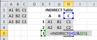
In the picture below, there are two sample tables. The one on the top left is my “Original Data Table” which could be stored on any tab. The “INDIRECT Table” on the right uses INDIRECT formulas to pull over the data from the first, original table.

INDIRECT1

Remember that the INDIRECT formula takes in a text string and converts it to a cell reference. In this case, I put my column references as table headers and my row references as row IDs for my INDIRECT table. In this second picture, you can see how I combine the column reference & row reference in my INDIRECT formula to create a formula that is easily copied over to all the other cells in my table.

INDIRECT2

With properly setup column & row references, I need only write a single INDIRECT formula to pull over all my data in the correct order. I could just have easily made it skip every other row or skip a couple of columns, or even reorder the columns or rows by reordering my column & row references. My INDIRECT formula wouldn’t have to change at all!

Hope this helps! Let me know if you have any further questions.

Thanks!
~Yosef

Excel: How to use the INDIRECT function


The Excel INDIRECT function is useful for displaying data in another cell by passing it text strings to tell it where the value is.

The syntax for the Indirect function is as follows:

INDIRECT(ref_text,[a1])

Where:

ref_text is a text reference to another cell & [a1] is a logical value that specifies what type of reference style ref_text is using.

In excel you have two types of cell reference styles:

  1. A1 style is where each row has a number and each column has a letter (the default view in excel).
  2. R1C1 style is where each row has a number and each column has a number.

A1 is indicated by [a1] = “TRUE”, R1C1 is indicated by [a1] = “FALSE” in the INDIRECT formula.

For example in order to display a specific column of data in a given row (in this example, row 7), the following function is used:

=INDIRECT($B$1&$A7,TRUE)

The first argument, $B$1&$A7 concatenates the values in cell B1 & A7 together to create a text statement of where the data that needs to be displayed is stored. In this case B1 = “Data!B”, A7 = 3 so the final result is “Data!B3” so the value displayed in the cell is the value on the Data tab in the B3 cell.

Column A now displays the row of the data for that particular project on the “Data” tab.

Hope you find this useful!

~Yosef

Excel: Formula Auditing – how to troubleshoot #N/A or #REF errors?


Excel comes with a handy tool called the “Formula Auditing tool” located on the Ribbon under the “Formulas” section under “Formula Auditing”.

(Click to Enlarge)
(Click to Enlarge)
  1. The Trace Precedents tool shows you visually which cells are used by the selected cell in it’s formula.
  2. The Trace Dependents tool shows you visually which cells are used by the selected cell in it’s formula.
  3. The Evaluate Formula tool walks you through the formula in the selected cell so you can see how it’s calculating the formula. If there is an error, this is a handy way of figuring out where the calculation goes wrong so you can potentially fix it.
(Click to Enlarge)
(Click to Enlarge)

Simple right? If not – feel free to leave a comment below & I’ll try to help!

~Yosef

How to Hide Pivot Chart Filters


(Directions below are for Excel 2010)

I recently built a simple dashboard using pivot tables with corresponding pivot charts. I was asked by my client if I could remove the filters from the pivot charts so that they would have a cleaner look for presenting. I had never worried about this before and didn’t know how off the top of my head so I did a couple of quick Google searches & couldn’t find any references on how to hide the filters! I was very surprised that I couldn’t find anyone else asking the question so I thought I would share how to easily do this. Luckily it’s pretty simple – I just didn’t realize these options existed!

Here’s a Pivot chart with the usual filters visible:

Pivot with Filters

To remove these filters, click the “Field Buttons” (or drop down for more control) button on the Analyze tab of the PivotChart Tools section of the menu ribbon (only visible if the chart is selected):

Pivot Chart Filter/Field Buttons

You can then choose which (if any) filters to display so that your chart looks nice & clean:

Pivot Chart w/o Filters

Hope this helps!

~Yosef B.